| Macroeconomic Consequences The decision to remove the American dollar from bimetallism in 1873 did not have immediate consequences,
for, as we've seen before, silver was undervalued at the legal
ratio and nobody used it anyway. But as one country after the other switched to the Gold Standard at the end of the century, the
demand for gold rose tremendously and a flow of silver was freed from monetary purposes in
France, England, Germany and most other big countries. (More
on this).
The result was that the dollar (and so the American
monetary mass and ultimately output and employment) was linked to a metal that was getting
scarcer and scarcer, because between 1879 and 1897 the rate of increase in gold output
slowed, and the demand increased at the same time. The monetary mass could not keep pace
with the strongly expanding economy, and price measured in gold declined strongly. This
deflationary effect was hindered to some extent by the spreading monetization of the
American economy and a more efficient banking system that allowed to pile up more paper
money on a given currency base (that is, gold). (more on this)
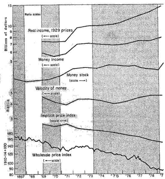
We see between 1875 and 1896 a deflation of about 1% a year in the general CPI. A the same time the output rose by 6 % a year.
Economists reader should not say, <<Gee what a growth even with those declining
prices!>>. It's precisely this growth that made the prices go down. With a
fixed quantity of money if the number of transactions rises and the velocity cannot rise
sufficiently, then prices have to fall.
All this led to a depression so great that you would
have to wait for 1932 to see the same again. Unemployment peaked at 18 % in 1894. But some
people suffered more than others (more on this).
On the monetary side, this deflation made many bank loans
turn sour, as the debtors struggled to honor their obligations with rising real value of
their debts. Some famous banking panics occurred (1892) , but globally the trust of the
public in the banking system increased. The ratio of deposits to reserves rose from 2 to 4
at the end of the period.
Next slide
NB : By clicking on words in the commentary, you will
be taken to the glossary where I have defined most of the specialized terms for you.
Please use your BACK button to come to the original page. |