Page 4 on 8 | Table of contents | Last | Next

.

A.

Dimensionality of the problem

Let's look at the cloud of point that stands for the rectangular figure table, the sum of whose column and rows we have transformed to one (that is, percentage). This cloud is contained in a space of dimension card(I)-1 or card(J)-1, whichever is lower. For the end of this paper we will assume that I<J and thus the problem is of dimension card(I)-1. In our example the table is 8x12 and is thus contained after its transformation in percents in a 7 dimensional space.

.

.

B.

Geometric principles

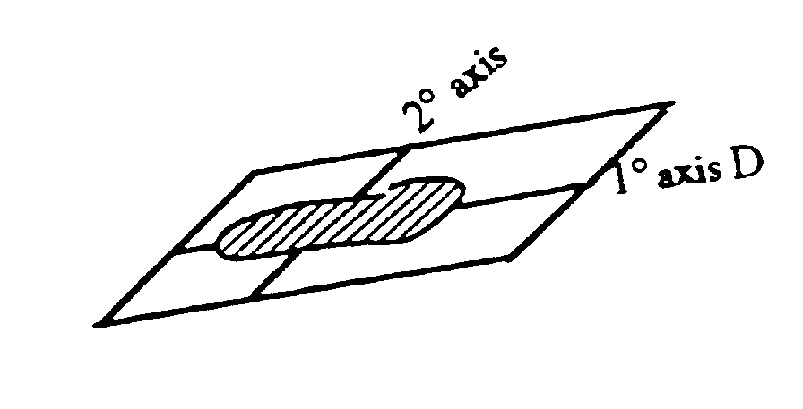
Basically, the insight of any factor analysis and in particular of correspondence analysis is that the cloud of points that we are trying to describe does not stretch equally in every direction, but on the contrary that it has a definite shape which is not an hyperball, for there is affinity between rows and columns. We are then going to define a new system of orthogonal coordinate more "economical".

More precisely, what we seek is for a cloud of points N(I) (remember that each point is located in space by its card(J) coordinates on J, that is, its profile on J) the representation which, in as small as possible a dimensionality (that is, the minimum number of axis), is as good as can be. If we want a graphical representation on paper, the problem can be formulated as follows : determine the subspace L of dimension 2 which pass through the center of gravity of the cloud (i.e. its mean profile) and which maximize the inertia of N(I) parallel to L. The softwares do not stop at 2 dimensions and you get in the standard output the card(I)-1 dimensions of the problem. But we have to be more general now.

.

.

C.

Factorial Axis

If we denote by any row which pass through the center of gravity of cloud N(I), we can break up the total inertia of the cloud in the sum of inertia parallel to (projected on) and inertia perpendicular to . The first factorial axis is row for which the inertia parallel to is maximum. The second factorial axis is, among all rows orthogonal to , the row for which the projected dispersion (inertia) of the cloud orthogonally complementary to is greatest ("What is left of inertia"). Going on axis after axis, we can extract factorial axis which make the new set of orthogonal axis in which the cloud can be totally described. These axes are called principal axis of inertia.

.

We seek for the cloud N(I) a representation as good as possible in a lower dimensional space. We project the cloud N(I) on a lower subspace L (a line, a surface, etc...) which pass through its center of gravity. The projection of the cloud on L will give us the approximate representation that we are looking for. On the picture on your left you see a flattened and cigar shaped cloud which stretches in the direction of axis D. The second axis is perpendicular to D. After all, factor analysis are nothing but a change of axis !

To each axis is associated an eigenvalue whose sum equals the inertia of the cloud. Each eigenvalue is worth 1 at most. You can see that if N(I) had only one point, there would be no axis, and if it had only 2 points, it would have a single axis; with 3 points we would need at most 2 perpendicular axis and for n points a maximum of card(J)-1 axis.

.

.

D.

Symmetry of both analyses

We have so far talked only about the analysis of one side of the table, rows or column.We can either project the row-points in the 11 dimensional community space or project the column points in the 7 dimensional schooling level space. We would then obtain 2 representations of the two cloud. Are these representations different ? Not much. The analyses are symmetric in three ways :

.

(1) As already shown, the clouds N(I) and N(J) have the same dimension (the rank of the matrix, here equal to 7) and are thus totally descriptible in a 7 axis system.

.

(2) It can be demonstrated that the eigeinvalues for this new set of axis is the same for both clouds.

.

(3) The column points projected in the analysis of row points appear in the same order but at a different scale in the other analysis. The proportionality coefficient is equal to the square root of the table's inertia.

.

Statisticians have decided not to differentiate between the two systems of factorial axis born from both analysis, and to represent all points on the same graph. The algorithm represent the points (see below how) in the space created by the k first factorial axis. The distance between points will be a distance to the mean profile (or centroid) in the Euclidean space of the paper sheet.

Besides the graphs, the softwares give us material to answer some of the scientist's questions like : Which part of the total inertia is accounted by the first k axis ? Which part of the variation of a given point is accounted by this particular graph ? What is the contribution of each point to the construction of the axis system ?

.

Next page : the output and how to interpret it